To process and analyze data for typical analytics or machine learning use cases, it is common to hit storage and processing power issues.
If the dataset is too big to be stored on your laptop drive, if it cannot be entirely loaded into memory, you must find practical solutions. It is, of course, possible to divide your dataset into smaller chunks, but that takes some time. And besides, you do not want to waste time waiting for a simple but non-scalable job to deal with lots of data.
These problems arise early: as soon as you start prototyping. Other problems arise once you have a working prototype, and would like to make it industrial. You are likely to have to partially or entirely rework your code or hope someone will do it for you to benefit from resiliency, monitoring, scalability.
Because the Punchplatform is production focused, these problems are important to us. If no data scientist can easily design applications to be deployed on a punchplatform where the real data is stored, what would be the point? To tackle that issue, we designed the Punch in a way easy to use and understand.
In this blog, we illustrate this using a simple example. First, we explain how we rely on Elasticsearch to make our input data easier to manipulate and easily distributed to a scalable machine learning pipeline. Second, we show how to transform a Jupyter notebook that does the job fine into an equivalent PML configuration. Interestingly this turns out to be very natural and easy to do.
We explain finally why altogether, you can quickly transform a smart Jupyter proof of concept into an industrial project and benefit from resiliency, monitoring, and scalability.
Dealing With the Input Data
We start with our dataset provided as a bunch of CSV files. We have 320Gb of these. Big enough to have troubles loading that into a simple notebook. Each file contains CSV AIS records. Here is an example:
#speed,category,ship_type
22, military, frégate
18, tourisme, catamaran
The first thing we do is to move that data into an Elasticsearch cluster. We will explain the rationale of this right next. To move the data to Elasticsearch you need a simple ETL pipeline: read the files, transform the CSV record into JSON document, then index it into Elasticsearch.
On the punch, you do that with a topology configuration file. The principle of a that is illustrated next.
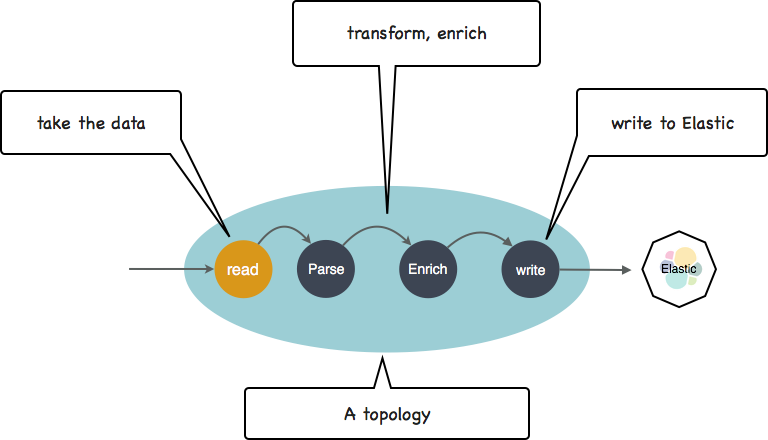
If you are familiar with Logstash (on an ELK), it is very similar: a plain configuration file to do the job. (if you are interested, check this documentation). In there you have a few lines of code to actually transform the CVS into JSON. Here it is.
{
    //The parsing operation
    if (!csv("speed", "category","ship_type").delim(",").on(message).into(tmp:[csv])) {
        raise("Parsing exception: not a valid  ais input");
    }
}
You can run that topology either from your terminal (just launch it), or (it is as easy) to submit it to a real Storm cluster. The point is : already that first step will benefit from scalability and high performance. It works with a few files, but also for terabytes of data.
What do you end up with? You now have your data properly indexed into Elasticsearch with two key benefits. First, you can visualize and search your input data using Kibana.
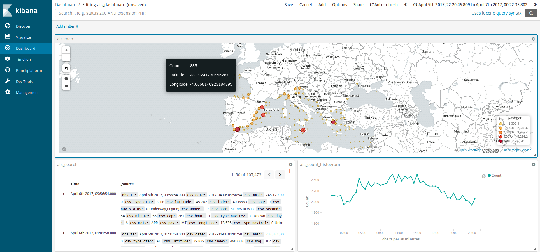
You will soon discover that Kibana, once mastered, is extremely powerful and easy to use, and gives you greater search power than simple notebook visualization capabilities. This is already a good starting point to think about your data and use cases.
Second, because Elasticsearch is a distributed database, it becomes simple to design a scalable machine learning pipeline to efficiently process your data on several servers. This is the next step we describe.
From a Python Notebook to a Spark Pipeline
This part requires you to be familiar with python and notebooks. To make it simple, here is the essential idea: notebooks make it very easy to design so-called pipelines that take your input data, apply the necessary transformations (filtering, enrichment, vectorization etc..), call some ready-to-use machine learning algorithms, and finally check and output the results.
In our case here is a quick view of our pipeline:
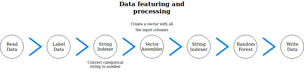
If you have a look at this document you have the complete notebook we started with. For now, we will simply focus on one of the steps in there. The one that actually invokes a random forest classification algorithm that really does the job of classifying a ship as a tanker or something else.
The way it works is simple: first you train it on some labeled data, then you can use it to classify new data, i.e. in our case guess the type of ship of each new AIS record.
Here is how all this looks like in our Jupyter notebook.
rf = RandomForestClassifier(labelCol="label_indexed", featuresCol="features_indexed", numTrees=100,
                            maxDepth=10, maxMemoryInMB=256, impurity='gini', featureSubsetStrategy='3')
df_tmp = rf.fit(df_tmp).transform(df_tmp)
In there, the fit() function call corresponds to the training, and the transform() call to the classification of new data. The various parameters you see in the RandomForestClassifier() function call are specific to that particular random forest algorithm.
The random forest input data with all the required variables is features_indexed. The label is in the label_indexed field. (These names were chosen by the developer).
Without going to more details, here is what the same step looks like using PML, the punchplatform machine learning pipeline format.
{
  "type": "org.apache.spark.ml.classification.RandomForestClassifier",
  "settings": {
      "labelCol": "label_indexed",
      "featuresCol" : "features_indexed",
      "numTrees" : 100,
      "maxDepth" : 10,
      "maxMemoryInMB" : 256,
      "impurity" : "gini",
      "featureSubsetStrategy" : "3"
  }
}
As you see, it is very similar. Instead of python code, you have JSON, but it stays as simple to read and understand. Other steps as similar. In the annex, we give explanations of each of them.
Putting it All Together
PML and the punchplatform are not designed to replace notebooks. However, combining notebooks with Elasticsearch and Kibana, and leveraging the punchplatform PML makes it simple to quickly start dealing with a large dataset and design pipelines that will make their way to production smoothly.
Besides, the end result stays readable and simple to understand. A PML file is just a configuration file. No code, no jars, everything is deployed on the platform as configuration files. It took us half a day to completely transcribe the notebook into PML.
The last benefit is to scale. If at the end you have a large dataset, having spark behind the scene helps a lot. In the punchplatform, this is what we have, lots of normalized data stored in big elasticsearch clusters.
Thank you for reading that article. The next posts will be about processing an unknown dataset and creating a new PML node based on a handmade algorithm. Stay tuned!
Annex
Here is a description of each processing step in PML and in the Notebook
Imports
Notebook
import findspark
findspark.init()

import pyspark
from pyspark.sql import SparkSession
from pyspark.ml.feature import IndexToString, StringIndexer, VectorIndexer, VectorAssembler
from pyspark.sql.functions import *
from pyspark.sql.types import FloatType, DoubleType, StringType, IntegerType, StructType, StructField
from pyspark.ml import Pipeline, PipelineModel
from pyspark.ml.classification import RandomForestClassifier, GBTClassifier
from pyspark.ml.evaluation import MulticlassClassificationEvaluator, BinaryClassificationEvaluator
PML
No import is needed.
Initialisation
Notebook
sc = pyspark.SparkContext(appName="PredNav_Cargo")
spark = SparkSession(sc).builder.master("local").getOrCreate()
PML
The Spark Context is already initialized. Using PML you are free from coding all these.
Prepare the data
Notebook
list_col = ["sog", "cap", "latitude", "longitude", "hour", "nav_status", "type_navire1"]
df = spark.read.parquet('dataset/mediterranee_0406_spark_sub.parquet').select(list_col)
df = df.withColumn("hour", df["hour"].cast("integer"))
PML
We have done that part in the topology.
Add a well-defined label
Notebook
class_pred = '7-Cargo'
df = df.withColumn('label',when(df.type_navire1 == class_pred, 'cargo').otherwise('other'))
PML
{
  "type": "punch_batch",
  "component": "labellisation_transform",
  "settings": {
    "punchlet_code":
      %%PUNCHLET%%
        {
        	String class_pred = "7-Cargo";
        	String type_navire1 = root:[csv][type_navire1].asString();
        	if (class_pred.equals(type_navire1)){
        		root:[label] = "cargo";
        	}
        	else{
        		root:[label] = "other";
        	}
        }
      %%PUNCHLET%%,
    "input_column": "source",
    "output_column": "labellisation"
  }
}
String Indexer
Notebook
nav_status_Indexer = StringIndexer(inputCol="nav_status", outputCol="nav_status_indexed").fit(df)
df_tmp = nav_status_Indexer.transform(df)
PML
{
   "type": "org.apache.spark.ml.feature.StringIndexer",
   "settings": {
     "inputCol": "nav_status",
     "outputCol": "nav_status_indexed"
   }
}
Vector Assembler
Notebook
features_col = ["sog", "cap", "latitude", "longitude", "hour", "nav_status_indexed"]
assembler = VectorAssembler(inputCols=features_col, outputCol="features")
df_tmp = assembler.transform(df_tmp)
PML
{
  "type": "org.apache.spark.ml.feature.VectorAssembler",
  "settings": {
      "inputCols": ["sog", "cap", "latitude", "longitude", "hour", "nav_status_indexed"],
      "outputCol" : "features"
  }
}
Vector Indexer
Notebook
feature_indexer = VectorIndexer(inputCol="features", outputCol="features_indexed", maxCategories=30)
df_tmp = feature_indexer.fit(df_tmp).transform(df_tmp)
PML
{
  "type": "org.apache.spark.ml.feature.VectorIndexer",
  "settings": {
  "inputCol": "features",
  "outputCol" : "features_indexed"
  }
}
String Indexer
Notebook
label_indexer = StringIndexer(inputCol="label", outputCol="label_indexed").fit(df_tmp)
df_tmp = label_indexer.transform(df_tmp)
PML
{
  "type": "org.apache.spark.ml.feature.StringIndexer",
  "settings": {
  "inputCol": "label_string",
   "outputCol": "label_indexed"
   }
}
Random Forest
Notebook
rf = RandomForestClassifier(labelCol="label_indexed", featuresCol="features_indexed", numTrees=100,
                            maxDepth=10, maxMemoryInMB=256, impurity='gini', featureSubsetStrategy='3')
df_tmp = rf.fit(df_tmp).transform(df_tmp)
PML
{
  "type": "org.apache.spark.ml.classification.RandomForestClassifier",
  "settings": {
  "labelCol": "label_indexed",
  "featuresCol" : "features_indexed",
  "numTrees" : 100,
  "maxDepth" : 10,
  "maxMemoryInMB" : 256,
  "impurity" : "gini",
  "featureSubsetStrategy" : "3"
  }
}
Saving the Output
PML
To end the process, we write the data to Elasticsearch, so as to check how well our pipeline works, and to perform further analysis.
{
  "type": "elastic_batch_output",
  "component": "output",
  "settings": {
    "index": "output-ais",
    "type": "log",
    "cluster_name": "es_search",
    "nodes": ["localhost"],
    "column_id": "id",
    "column_source": "output"
  },
  "subscribe": [
    {
    "component": "mllib",
    "field": "data"
    }
  ]
}