Introducing OmniSci

Before diving into leveraging OmniSci, let us quickly recap the well-known database story.

Relational databases have long been the standard for storing pre-processed data. Although they cannot keep up with today’s applications requirements in terms of raw performance and volumetry, they stay by far the most popular and the most widely used databases. Their low learning curve still makes them a popular choice.

With applications becoming more and more data-centric, the amount of data increased dramatically. A new era then started: NoSQL or NotOnlySQL. Instead of relying on a single server for computation and disk I/O, NoSQL databases started to extensively rely on parallelism and sharding, i.e. multiples servers are used to fulfill the computation needs. Distributed filesystems and the map-reduce ecosystem also became popular to deal with Tb or Pb of data. Variants of SQL re-appeared on top of these to provide developers with higher-level APIs. Although it is overly simplified, it is common to refer that whole trend as “Big Data”.

Big Data gave us all some respite… until artificial intelligence came in. Developers now expect to have at hand many great algorithms to apply machine learning and deep learning processing to their data. These algorithms unleash lots of great use cases: classification, predictive analysis, pattern recognition, image processing etc..

CPUs alone are not powerful enough to deal with these use cases. Vectorized data, which are widely used in deep-learning and machine-learning algorithms require GPU power. Not to say that if you mix big data and deep learning you end up with distributed GPU clusters.

Without surprise, GPUs capable databases are now entering the game.  In this post, we introduced one of these new player: OmniSci, and we provide a walkthrough guide for you to combine it with the Punchplatform.

Introducing OmniSci

OmniSci (formerly Mapd)  is an in-memory columnar SQL engine designed to run on both GPUs and CPUs. OmniSci supports Apache Arrow for data ingest and data interchange via CUDA IPC handles.

Some features that distinguished MapD from its competitors are:

• built-in interface for data exploration and data visualization (GeoSpatial data)
• built-in algorithms and functions to manipulate GeoSpatial data
• makes use of both CPUs and GPUs instead of CPUs only
• a low learning curve
• .. and SQL of course

The PunchPlatform now integrates OmniSci into its ecosystem. Let us see how we can put all of this into play on a (16.04LTS) ubuntu server.

WalkThrough : The Basics

GPU driver Installation

To start with, you need GPUs. Here is how to setup your environment on a NVIDIA equipped laptop. Of course this may be skipped if you have a cloud GPU box ready.

You first need to install the NVIDIA CUDA Toolkit for application development. Download the DEB package from the  NVIDIA CUDA zone.
Install the CUDA repository, update local repository cache, and then install the CUDA Toolkit and GPU drivers:

$ sudo dpkg --install cuda-repo-ubuntu1604_8.0.44-1_amd64.deb
$ sudo apt update
$ sudo apt install cuda-drivers linux-image-extra-virtual
$ sudo reboot

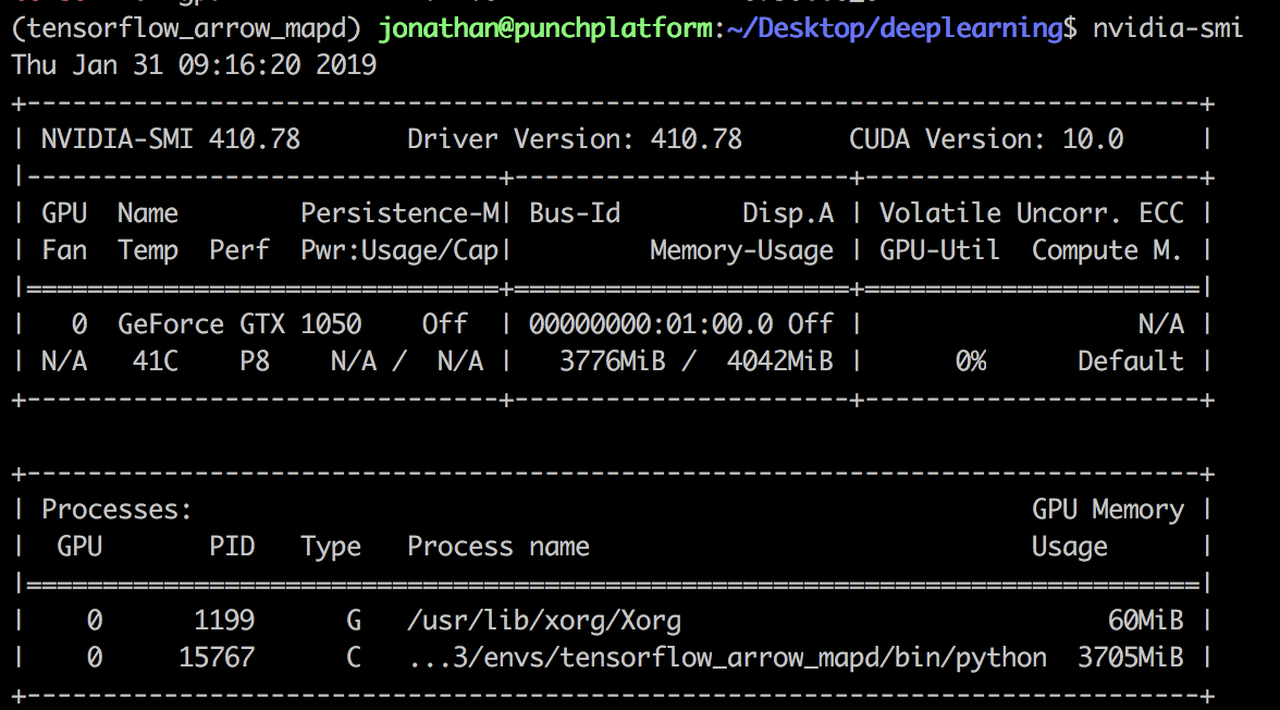
Check the installation of the GPU drivers by running the following command:

$ nvidia-smi

Install OmniSci 

Download OmniSci here. Use the .targz for this tutorial. Starting MapD (the database itself) is as simple as:

$ cd $YOUR_MAPD_DIR 
$ ./startmapd

Inserting Data

To insert data, we will set up a punchplatform topology. The punch 5.2.1 version now includes a mapd bolt which makes it easy to feed MapD with any data coming from the many possible punch data sources: Kafka, files, sockets, whatsoever.

We assume you are already familiar with the PunchPlatform.  In short, it lets you design Storm or Spark pipeline using simple configuration files. These files can now include a MapD connector, hence MapD is just one of many possible data sink in the PunchPlatform.

Here is how it works: the MapD bolt is inserted as a sink in a (storm) DAG (Directed Acyclic Graph) and receives its data from a spout or previous bolt.  It expects a valid flat K-V (Key-Value) map. In other words, a row in your database is represented as a map object where the key corresponds to the target SQL column name.

Note that when you insert data into MapD, you can also include Geo-Spatial primitives  (see this link for a complete list). For instance, given the following table:

create table mytable (aPolygon polygon)

You can insert a polygon using the POLYGON primitive inside your insert SQL query statement:

insert into mytable values ('POLYGON((1 2,3 4,5 6,7 8,9 10))');

To see and check your data :

select * from mytable;

Let us see a punchplatform topology example that will fill MapD with automatically generated geolocation points.  This topology uses the Generator Spout to generate the data, forwarded to the MapD bolt to insert it into MapD. We also added a punchlet (embedded in the topology using the Punch Bolt). Punchlets are handy to refine and enrich the data in your pipelines, which is a fundamental step in a real-world scenario.

Here is the topology:

{
  "spouts": [
    {
      "type": "generator_spout",
      "spout_settings": {
        "interval": 0,
        "messages_count": 99,
        "messages": [
          { "logs": {  
               "name": "tom%{message_num}", 
               "surname": "jerry%{message_num}", 
               "ip" "%{message_num}.%{message_num}.%{message_num}.%{message_num}" 
            }
          }
        ]
      },
      "storm_settings": {
        "component": "generator"
      }
    }
  ],
  "bolts": [
    {
        "type" : "punch_bolt",
        "bolt_settings" : {
           "punchlet" : "./mapd.punch"
        },
        "storm_settings" : {
          "component": "aggregate_data",
          "subscribe": [
            {
              "component": "generator",
              "stream": "logs"
            }
          ],
          "publish" : [
              { 
                "stream" : "logs", 
                "fields" : ["name", "surname", "age", "lon", "lat", "ip", "geolocation"] 
              }
          ]
        }
    },
    {
      "type": "mapd_bolt",
      "bolt_settings": {
        "host": "localhost",
        "username": "mapd",
        "port": 9091,
        "password": "HyperInteractive",
        "database": "mapd",
        "bulk_size": 3,
        "insert_type": "thrift_transport",
        "table": "fake_data",
        "column_names": [
          "age",
          "name",
          "surname",
          "geolocation",
          "ip",
          "lon",
          "lat"
        ]
      },
      "storm_settings": {
        "executors": 1,
        "component": "mapd",
        "subscribe": [
          {
            "component": "aggregate_data",
            "stream": "logs",
            "fields": [
              "age", "name", "surname", "geolocation", "ip", "lon", "lat"
            ]
          }
        ]
      }
    }
  ]
}

And here is the punchlet:

  // Generate random number between 0 - 100
  [logs][age] = (int)(Math.random()*100);
  
  // We are going to deduce longitude and latitude from IP address 
  Tuple result;  
  if (geoip().on(root:[logs][ip]).into(result)) {
    // if our parser successfully deduce a longitude and latitude
    [logs][geolocation] = "POINT(" + result:[longitude].toString() + " " + result:[latitude].toString() + ")";
    [logs][lon] = result:[longitude];
    [logs][lat] = result:[latitude];
  } else {
    // in every other scenario assign a fake value
    [logs][geolocation] = "POINT(0 0)";
  }
}

What it does is to determine geolocation from the IP address and format our data stream to a valid one. Notice the insertion of the MapD POINT primitive.

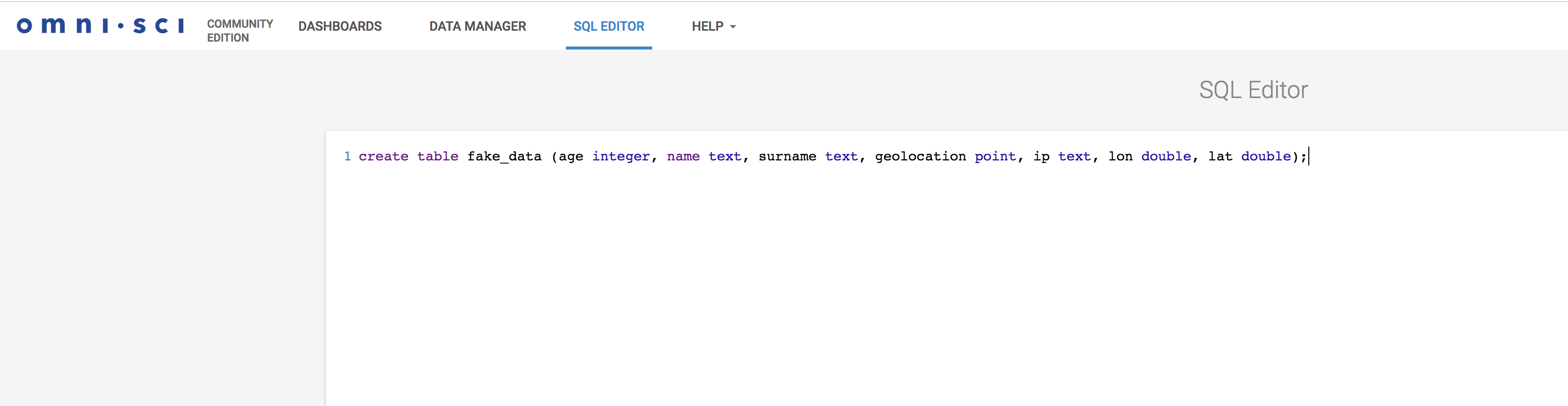
To create the table, we will use the OmniSci Immerse. Immerse is for OmniSci is what Kibana is for ElasticSearch. It also includes a SQL editor to create tables and execute arbitrary SQL statements. It looks like this.

Once the table is created, simply run the topology: (here mapd.json is your topology filename)

$ punchplatform-topology.sh -m light -t mapd.json

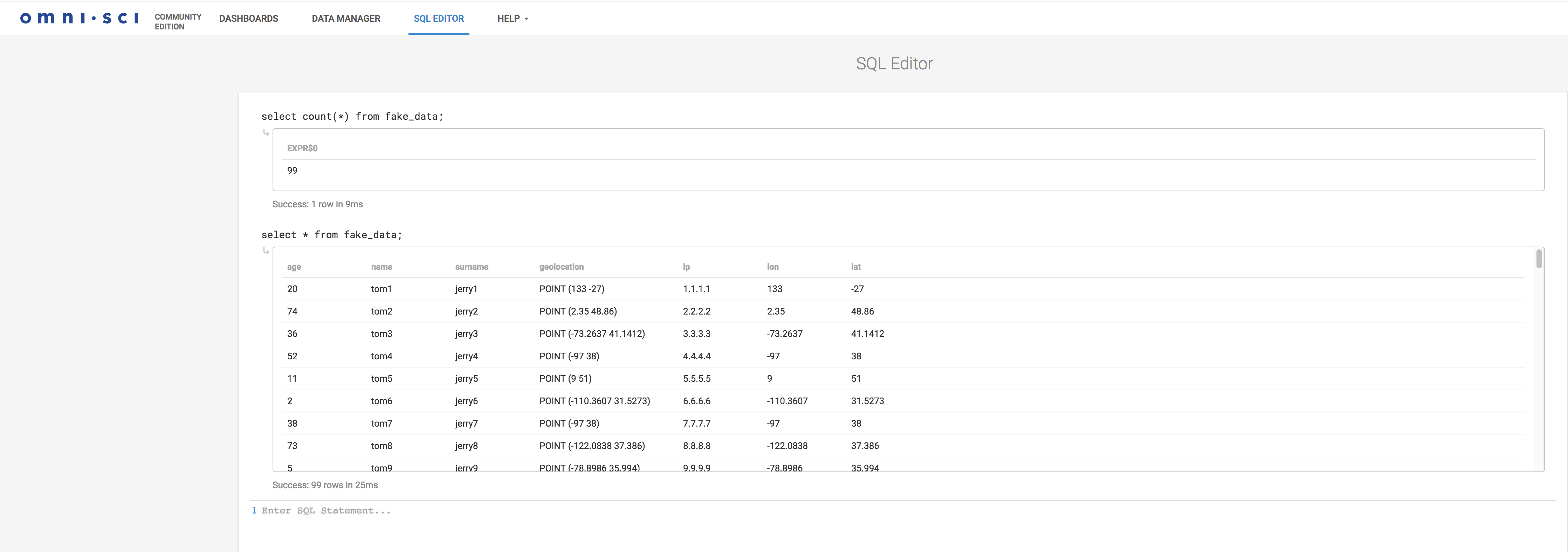
You can now query the data, again from the SQL editor:

select count(*) from fake_data;
select * from fake_data;

Visualise Your Data

Now that the data is in,  we can create visualizations. Here is an example histogram setup in a few clicks. It is somehow similar to the Kibana experience: straightforward.

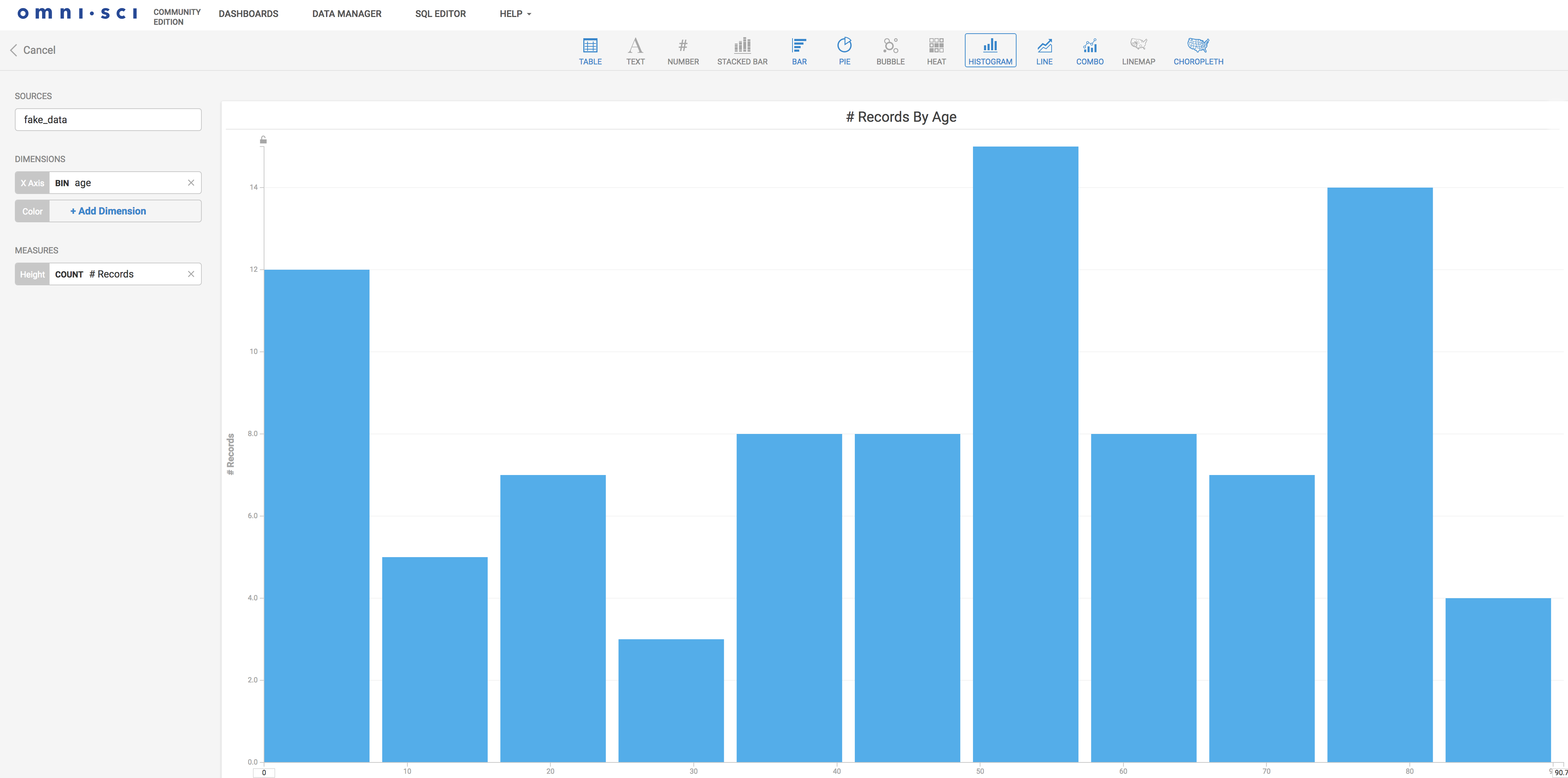
Here we are displaying the frequencies of the inserted data age distribution. OmniSci Immerse can do much richer and powerful visualizations, checkout examples of what can be done here.

WalkThrough: Machine Learning and TensorFlow

This part is subtle, we hope you can stick with us until the end of this blog. It gives a first sense of going datascience with OmniSci.

Before that a few words on Apache Arrow that is in the picture:

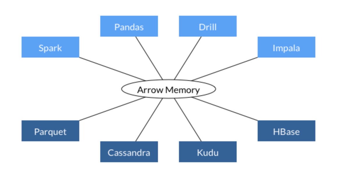
Apache Arrow is a cross-language development platform for in-memory data. It specifies a standardized language-independent columnar memory format for flat and hierarchical data, organized for efficient analytic operations on modern hardware. It also provides computational libraries and zero-copy streaming messaging and interprocess communication. Languages currently supported include C, C++, Java, JavaScript, Python, and Ruby.

In short,  Apache Arrow is used as a core component in many big data components (Spark, Tensorflow, OmniSci, etc…) for data interchange.

What we will try to achieve in our next part is something similar to the code below:

import tensorflow as tf
import pandas as pd
import pymapd
import pyarrow as pa

# tell tensorflow to use the first GPU of your machine
with tf.device('/GPU:0'):
    # use your pandas/pymapd in-memory GPU data with tensorflow
    # here you should start training some models...
    myTensorData1 = pa.read(your_dataset_in_gpu_memory)
    # do something

We will also use Anaconda, well-known python package used for data manipulation. It comes with handy features, in particular, the Jupyter Notebook. Grab anaconda installation script for Ubuntu and restart terminal after installation:

wget https://repo.continuum.io/archive/Anaconda3-2018.12-Linux-x86_64.sh
./Anaconda3-2018.12-Linux-x86_64.sh
source ~/.bashrc

Make sure none of your conda environment is currently activated:

conda deactivate

Now, we are going to configure our anaconda working environment by executing the commands lines below: We are going to create fresh python virtual environment by using anaconda cli (conda):

conda create --name mytensorflow_env python=3.6
conda activate python3_tensorflow
python3 -m ipykernel install --user --name mytensorflow_env --display-name "python 3 tensorflow"
conda activate mytensorflow_env

Once you made sure the environment is created (your virtualenv name will appear on your terminal), installs the python libraries below:

conda install tensorflow-gpu 
conda install ipykernel conda install -c conda-forge pyarrow 
conda install -c nvidia -c rapidsai -c numba -c conda-forge -c defaults cudf=0.4.0 
conda install -c conda-forge pymapd conda install matplotlib 
conda install -c conda-forge tensorboard
conda install pandas

For debugging purpose you may want to list all your virtual environment by using:

conda env list

or if you want to see the list of installed libraries in your conda virtual environment:

# solution 1
conda list

# or solution 2
python -m pip list

Note:

you might want to install pandas, numpy, etc… just use conda install XXX where XXX is the name of the package you want to install

Using TensorFlow

Test in jupyter if everything is working – don’t forget to set the python kernel to the one you just created: python 3 tensorflow

In your Jupyter Notebook, run the codes below:

import tensorflow as tf
hello = tf.constant('Hello, TensorFlow!')
sess = tf.Session()
print(sess.run(hello))

Running the above code should display as result: Hello, TensorFlow!

Now, let’s try to fetch some data inside our GPU memory. Here comes Arrow into play. (checkout OmniSci blog for details).

First we check that pymapd and MapD are properly installed on our  GPU by executing the code below in Jupyter:

import pandas as pd  
import sys  
from pymapd import connect

con = connect(user="mapd", password="HyperInteractive", host="10.35.6.106", dbname="mapd", port=9091)  

Once you passed that step above, grab the tab-delimited PUF dataset here: download. Note that you might want to take only a subset of the downloaded data for your test.

use head -1000000 download_file.txt >PartD_Prescriber_PUF_NPI_15.txt

Load the  data  into a pandas dataframe (change host, password, user, dbname, port parameters accordingly to yours):

import pandas as pd  
import sys  
from pymapd import connect

con = connect(user="mapd", password="HyperInteractive", host="10.35.6.106", dbname="mapd", port=9091)  
prescriber_df = pd.read_csv('PartD_Prescriber_PUF_NPI_15.txt', sep='\t', low_memory=False)  
prescriber_df.head()

Your Jupyter notebook should now display a bunch of results.

Note:

The handling of nulls is crucial when working with pandas and MapD…

Finally, the code below shows how to remove N.A values from a pandas dataframe and save it a MapD database.

And at last, we display how to load data from a MapD database directly to GPU memory by using Arrow.

import pandas as pd  
import sys  
from pymapd import connect

# create a connection with MapD
con = connect(user="mapd", password="HyperInteractive", host="localhost", dbname="mapd", port=9091)

# load data into a pandas dataframe
prescriber_df = pd.read_csv('PartD_Prescriber_PUF_NPI_15.txt', sep='\t', low_memory=False)
# replace all NA values with 0
str_cols = prescriber_df.columns[prescriber_df.dtypes==object]  
prescriber_df[str_cols] = prescriber_df[str_cols].fillna('NA')  
prescriber_df.fillna(0,inplace=True)
# create a new cms_prescriber table into MapD and insert all data
con.execute('drop table if exists cms_prescriber')  
con.create_table("cms_prescriber",prescriber_df, preserve_index=False)  
con.load_table("cms_prescriber", prescriber_df, preserve_index=False)
# load data from MapD to GPU memory
df = con.select_ipc("select CAST(nppes_provider_zip5 as INT) as zipcode, sum(total_claim_count) as total_claims, sum(opioid_claim_count) as opioid_claims from cms_prescriber group by 1 order by opioid_claims desc limit 100")
# print the result
print(df.head())


# tell tensorflow to use the first GPU of your machine
with tf.device('/GPU:0'):
  a = tf.constant([1.0, 2.0, 3.0, 4.0, 5.0, 6.0], shape=[2, 3], name='a')
  b = tf.constant([1.0, 2.0, 3.0, 4.0, 5.0, 6.0], shape=[3, 2], name='b')
c = tf.matmul(a, b)
# Creates a session with log_device_placement set to True.
sess = tf.Session(config=tf.ConfigProto(log_device_placement=True))
# Runs the op.
print(sess.run(c))

It is now up to you to try some coding – i.e feed data from MapD to tensorflow by using GPU only memory.

Hope you enjoy this small ride 🙂 !